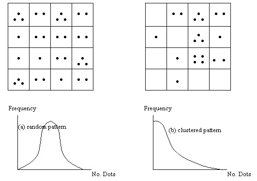
SETTING GUIDELINES FOR LIFTING THE BAN ON THE GREENBELT ZONESProf. Chulmin JUN, KoreaKey words: Greenbelt, RDZ, GIS, AHP, overlay. 1. INTRODUCTIONRestricted Development Zones (RDZ) which are established around the urban areas are intended to prevent urban sprawl and to protect natural environment. Ever since the policy was first introduced in 1971 in Korea, RDZ have been designated and maintained around 14 urban zones including Seoul metropolitan area. The areas sum up to 5,397 (5.4% of the total nation) and accommodate some 250,000 people. For three decades, many partial actions have been taken to make the rules less strict due to resistance from the residents in RDZ with the reason of inequality in living conditions and land values. Since 1999, however, the government has been presenting with series of radical changes in RDZ policy to abolish or modify the zone boundaries. The Korean Ministry of Construction and Transportation set up plans to free seven small- and medium sized urban areas which are under less development pressure from all restrictions on development and to partially adjust the zone boundaries in seven large cities including Seoul. Apart from the zones to be totally freed from restrictions, the problem, however, is how to partially demarcate the areas to be abolished or alleviated among RDZ in larger cities. Although the government says it will perform thorough and scientific evaluation on the concerned areas through experts-participating plans, no clear blueprints have been issued until now. The basic framework of the plan is designed to free large-sized existing villages with the population of 1000 or more from restrictions while partially lifting the restrictions on scattered groups of households which are not large enough to be totally freed. However, selecting portions in RDZ and drawing boundaries on them which have no visual marks will justifiably bring about a great deal of resistance and conflicts. The initial step should be devising strategies that can minimize such problems before implementing regulation measures. The methodologies should include means to incorporate many different aspects of decision elements and stakeholders' interests while being as subjective as possible. This study presents strategies to choose groups of residents in RDZ by employing the concentration index of them and means to incorporate preferences among different decision factors using the AHP method. 2. METHODS FOR THE ANALYSIS ON SPATIAL CLUSTERINGIt is viewed that partial relaxation will primarily be based on how many and how densely existing households are placed in the RDZ. The process will need to involve the steps for differentiating those residential areas from other part. This section presents reviews on existing approaches relating to analyses for dot-distribution patterns and presents a relevant strategy that can now be practically applicable to RDZ adjustment processes. 2.1 Quadrat AnalysisQuadrat analysis is represented by the probability density function that describes the number of objects placed in a grid of a space (Lee 1989, Thomas 1977). The given space is first divided into grids of same shape and size and the number of dots that belong to each grid are counted. As shown in Figure 1, the Quadrat Analysis classifies type (a) as random pattern and type (b) as clustered pattern using the ratio of variance to the mean. If the pattern is completely regular where each grid holds the same number of dots, the ratio becomes 0. The ratio becomes larger as the dots become concentrated on smaller number of grids with variance increasing.
Figure 1. The Quadrat Analysis The drawback, however, is that the same dot distribution pattern can be classified into either random pattern or clustered pattern depending on the size of the unit grid. Also, although this method helps to understand the degree of concentration of dot-distribution in the study area, it does not provide means to select those clustered portions. 2.2 Nearest-Neighbor AnalysisNearest-Neighbor Analysis describes the
distribution pattern using the distance of the nearest two points (Lee
1989, Getis 1964). It compares the actual mean distance (
where di is the distance of two points and n is the number of dots.
where The Nearest-Neighbor Index R is described by the ratio of these two.
R has a value from 0 to 1, being 1 in case of completely random distribution and 0 when the dots are concentrated on one point. Nearest-Neighbor Analysis has merit over Quadrat Analysis in that it is not affected by the size of unit grid, but its major drawback is that the result varies depending on the size of study area. Similarly to Quadrat Analysis, it is a method to measure the concentration degree of dots among the given space and cannot be applied to differentiating the concentrated area from other parts. 2.3 Overlap AnalysisContrast to the previous approaches which use either the number or distance of dots to calculate the degree of concentration in the study area, Overlap Analysis uses overlapped areas created by unit circles centering around randomly distributed dots and the mean distance of them (Koh 1995). Overlap Analysis analyzes the distribution of dots by calculating the ratio of total overlapped area to the total area of unit circles as follows.
where N is the number of dots and ri is the mean half distance of two points.
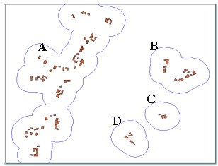
where C is the overlap index, P the sum of overlapped areas, V the summed area of unit circles, and the overlapped area Ai belongs to ni number of circles. The overlap index C becomes 1 when entire points are placed in one spot while 0 in case of the random distribution. 2.4 Using Buffering on the Overlap AnalysisThe methods discussed so far all deal with how much the entire dots in a given space are clustered and not how they are visually circumscribed or demarcated, which is the major concern in actual lifting processes in RDZ. For such purpose, we can use the buffering function that most GIS packages provide. As shown in Figure 2, we can easily draw polygons around existing buildings by using the buffering function with user-specified set-off distance. Polygon areas vary depending on the input radius resulting in different grouping such as A, B, C and D in the figure. For example, we can group B, C and D into one using longer buffer-radius or exclude some small groups according to decision strategies. Apart from grouping of buildings, the steps are required to analyze how densely buildings are placed in each group. By doing so, we can compare similarly grouped villages based on their concentration densities and, thus, can provide more validity in selecting the villages to be freed or alleviated from restrictions.
Figure 2. An example of grouping houses using the buffering function of the GIS
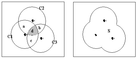
Figure 3. Buffering of dots and the concentration index The idea that was discussed in Overlap Analysis method, which is based on the overlapped areas of unit circles, can be modified and applied to establishing clusters of houses using the GIS-buffering. Figure 3 shows (a) the overlapping of buffered circles and (b) the cluster polygon that circumscribes them. If we follow the formula (4) and (5), the ratio of the total overlapped areas (2(S(a)+S(b)+S(c))+3S(d)) to the sum of the buffered circles (S(C1)+S(C2)+S(C3)) becomes as follows. However, this formula has a defect in that it generates same value 1 when the participating dots are placed in one spot regardless of the number of them. Since we should regard a resulting polygon (i.e. S in Figure 3) from the buffer operation as being more densely populated as it contains more dots in it, we should modify the current denominator which is the aggregation of circles to the entire polygon. Also, the numerator needs to change to the aggregation of each overlapped area multiplied by the number of overlaps taken place regarding to it as follows. By calculating the ratio of the sum of overlapped areas (taking into account the number of overlaps for each overlapped area) to the entire polygon resulting from dot-buffers, we can understand how densely houses are gathered in their clusters. This idea can be generalized as follows.
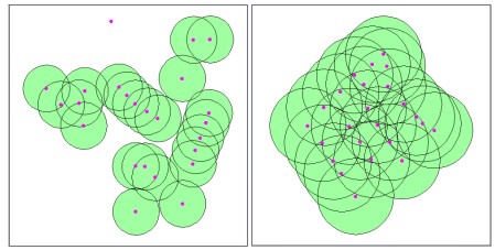
where the overlapped area Ai multiplied by ni–times of overlaps and S is the union area of buffered circles. The concentration index C generated from this formula becomes 0 in case of having no overlapped areas and N-1 when N buffered circles are fully overlapped, that is, all N dots are placed in one spot. If we assign concentration indexes to the buffered polygons as one of their attributes, we can compare the residential clusters based on these values. For example, polygon S in Figure 3 may have 0.5 as its attribute. Two residential clusters with the same number of households are compared in Figure 4 based on their concentration indexes.
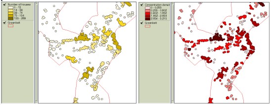
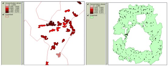
Figure 4. Concentration degrees of two clusters with the same 23 houses This methodology was applied to a portion of an actual RDZ to generate buffered zones and their concentration indexes as illustrated in Figure 5. 3. Composite Analysis3.1 Generating development-priorities using the overlayIn order to analyze the ‘developability’ or the priority for restriction-lifting among the clusters of houses, different decision factors should be taken into account. Not only should the decision making include various factors such as slope, elevation, distance to CBD, distance to highway/railroad, land price and environmental protection, but it should take into account that each of them has different importance or weight value. If we assume that more physical and environmental elements a site satisfies, more developable it becomes, the overlay function of GIS can be effectively applied to such problems.
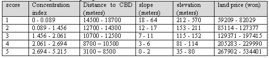
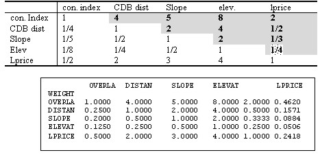
Figure 5. Creating buffers and displaying them based on the concentration index The development priorities can be obtained by using overlay function to find areas that satisfy decision criteria and then to overlay these areas with residential clusters that are created from buffer analysis. If each of decision criteria is categorized and assigned scores accordingly, the resulting overlaid map contains the aggregated scores, which represent the weight value for development or restriction-easing. Table 1 illustrates how decision elements are classified and assigned scores. This example assigned scores to different classes in proportion to their areas. Table 1. An example of assigning class scores based on class areas It is practical to assign different weight values to decision criteria since they have different importance each other. A technique in MCDM field called the AHP(Analytical Hierarchy Process) can be effectively used in comparing and prioritizing multiple criteria. The AHP which was developed by Saaty (1980) is a decision analysis technique used to evaluate complex multi-attributed alternatives. The AHP employs a systematic procedure for representing the elements of a problem hierarchically, enabling the subproblems to be easily evaluated. Simple pairwise comparisons are used for developing priorities in each hierarchy. Theoretical background of the AHP can be found in voluminous literature (e.g. Yager 1979, Saaty and Kearns 1985, Saaty 1980, 1987, 1990), and, hence, will not be discussed here. Table 2 illustrates how prioritized values are assigned based on the pairwise method and input to matrix for the calculation of entire weight values. Figure 6 shows a computer output containing the final weight values. Table 2. Prioritizing process using the pairwise comparison
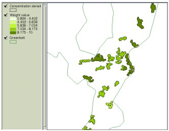
Figure 6. Calculation of weight values using the AHP Physical criteria can now be multiplied by weight values before they participate in overlay process and then the resulting map contains aggregated scores where different importance is reflected. Figure 7 displays the residential clusters having 20 or more houses according to aggregated weight values.
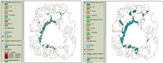
Figure 7. Aggregated weight values of clusters having 20 or more houses. Weight values can also be regarded as ‘looseness’ for condition variation in each decision criteria. Decision criteria with higher weight values can be viewed to play more critical role than others among the criteria included in overlay operation, which means condition modification of that criteria becomes more difficult or ‘dangerous’ than others. For example, Figure 8-(a) illustrates the areas having conditions of slope 6% or more, elevation below 80 meters, distance less than 1.3 km to CBD, and over 150000 won as the land price per pyung (1 pyung approximately equals to 3.3 m2). If the total area is not large enough and, thus, conditions need to be adjusted, weight values can be applied in loosening the conditions. Figure 8-(b) now displays loosened conditions with slope less than 10%, elevation less than 100 meters, distance less than 1.4 km to CBD and over 150000 won as the land price per pyung.
Figure 8. Using the weight values for loosening the constraints We must note that the AHP does not provide mathematically rigorous results and is a technique that helps systemize objective evaluations. Although the AHP does not yield exact numbers for the priorities of decision criteria, it can effectively help accommodate and adjust ideas from multiple decision makers. 4. CONCLUSIONSLifting RDZ restrictions is one of the most difficult problems that Korean government must tackle with. We can easily foresee complaints from the RDZ residents during the processes of choosing the areas to be freed from restrictions. One way to minimize them will be to establish strategies that are consistent and reasonable, which, however, will never be easy. With these issues in mind, this study presented that concentration index can be adopted as a tool to evaluate or choose residential clusters. Along with this, using the AHP technique was introduced in prioritizing multiple decision factors comprehensively. Of course, such techniques also require steps to set up some forms of principles. For example, providing different buffer distances yields different forms and numbers of residential clusters and setting different scoring schemes generates different scores in the final integration. Also, such steps would be required to determine how many classes are needed in the attribute values or where to divide the classes. These are some of the problems to be handled in the future study and yet it is viewed that the proposed techniques including the concentration index and the AHP in the GIS environment help decision makers in creating and comparing different alternatives. By refining and improving the techniques, planners will be aided in narrowing down wide discrepancies among stakeholders. REFERENCESGetis, A., 1964, Temporal land use pattern with the use of Nearest Neighbor and Quadrat Methods, Annals of the Association of American Geographers, Vol. 54. Koh, T., 1995, Analysis of dot-distribution and spatial relationships using Overlap Analysis, M.S. Thesis, Hanyang University. Lee, H. Y., 1989, Geographical Statistics, Seoul, Korea: Bupmunsa Pub. Saaty, T. L. and K. P. Kearns, 1985, Analytical Planning, Oxford, U.K: Pergamon Press Ltd. Saaty, T. L., 1980, The Analytical Hierarchy Process: planning, priority setting, resource allocation, New York: McGraw-Hill. Saaty, T. L., 1987, The analytic hierarchy process-what it is and how it is used, Mathematical Modelling, 9, 161-176. Saaty, T. L., 1990, How to make a decision: the analytic hierarchy process, European Journal of Operational Research, 48(1), 9-26. Thomas, R.W., 1977. An introduction to Quadrat Analysis, Concepts and techniques in modern geography No.12, Norwich: Geo. Abstracts. Yager, R. R., 1979, An eigenvalue method of obtaining subjective probabilities. Behavioral Science, 24, 382-387. CONTACTProf. Chulmin Jun 25 April 2001 This page is maintained by the FIG Office. Last revised on 15-03-16. |
||||||||||||||||||||
 ,
(1)
,
(1) ,
(5)
,
(5)